Download
The OSIRIS Level 2 and Level 3 data are available at our sftp server and require the following username and password:
- u: osirislevel2user
- p: hugin
The European Space Agency (ESA) asks that you use the data free of charge and obligation once you have completed a registration form outlining your area of research, etc. ESA keeps track of the number of registered users and uses this information to justify continued funding of the Odin mission. ESA funds the Odin satellite as a 3rd party mission and they ask that all data users be registered with them. Unfortunately the process uses a standard form for all third party missions which by itself is harmless, except they ask questions that unsettle many people. As an OSIRIS data user you are not required to provide any yearly reports of any kind to ESA even though the application forms asks you to agree to this after your application is submitted.
Additionally, the OSIRIS Level 2 data products are available via https through Globus. Transfer a single file or the entire collection of datasets easily with Globus.
If you are having trouble locating the data you are interested in, contact Taran Warnock.
OSIRIS Level 2 Data Products
Level 2 data users are ecouraged to read the User Guide for the data products.
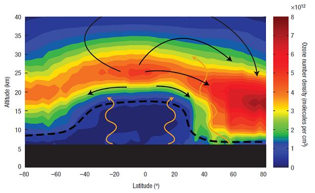
OSIRIS spectra of limb scattered sunlight are used to retrieve ozone number density vertical profiles over the altitude range from 10 to 60 km at a vertical resolution of approximately 1.5 km using the a Multiplicative Algebraic Reconstruction Technique, which is a one dimensional modification of a two-dimensional tomographic retrieval algorithm. This technique allows for the consistent merging of the absorption information from radiance measurements at wavelengths in the Chappuis and the Hartley-Huggins bands at each iteration of the inversion. A set of weighting factors is used to determine the importance of each line of sight and each element of the measurement vector for the retrieved state at each altitude. Retrieval algorithm details can be found in Degenstein et al., 2009.
The current version of the ozone product is version 5.10, which implements a tangent altitude registration correction algorithm to correct a small long term drift. See Bourassa et al., 2018.
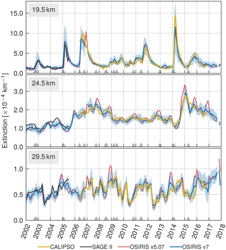
OSIRIS limb scattered sunlight spectra are used to retrieve vertical profiles of stratospheric aerosol extinction at 750 nm. All the spectra obtained with a single vertical scan of the spectrograph line of sight are used together to retrieve an extinction profile with approximately 1.5 km vertical resolution. Hydrated sulphuric acid particle microphysics, including a size distribution for typical background aerosol, are assumed to calculate the scattering cross section and phase functions required to retrieve the aerosol extinction. Fundamentals of the retrieval algorithm are detailed in Bourassa et al., 2012.
The current version of the stratospheric aerosol extinction is version 7.2. The user guide and examples are here. See details in Rieger et al., 2019. This version uses multiple wavelengths to reduce measurement geometry biases and improve extinction retrieval in the upper troposphere and lower stratosphere. The Chen et al., 2016, cloud detection algorithm has been adapted for the OSIRIS wavelength range for improved cloud screening and polar stratospheric cloud detection.
A new retrieval algorithm for OSIRIS (Optical Spectrograph and Infrared Imager System) nitrogen dioxide (NO2) profiles has been validated. The algorithm relies on spectral fitting to obtain slant column densities of NO2, followed by inversion using an algebraic reconstruction technique and the SaskTran spherical radiative transfer model (RTM) to obtain vertical profiles of local number density. The validation covers different latitudes (tropical to polar), years (2002–2012), all seasons (winter, spring, summer, and autumn), different concentrations of nitrogen dioxide (from denoxified polar vortex to polar summer), a range of solar zenith angles (68.6–90.5°), and altitudes between 10.5 and 39 km, thereby covering the full retrieval range of a typical OSIRIS NO2 profile. The use of a larger spectral fitting window than used in previous retrievals reduces retrieval uncertainties and the scatter in the retrieved profiles due to noisy radiances. Improvements are also demonstrated through the validation in terms of bias reduction at 15–17 km relative to the OSIRIS operational v3.0 algorithm. The diurnal variation of NO2 along the line of sight is included in a fully spherical multiple scattering RTM for the first time. Using this forward model with built-in photochemistry, the scatter of the differences relative to the correlative balloon NO2 profile data is reduced.
The NO2 data is available by following the directions under Download and navigating to the directory /OSIRIS/Level2/no2/
A 7+ year (2001–2008) data set of stratospheric BrO profiles measured by the Optical Spectrograph and Infra‐Red Imager System (OSIRIS) instrument, a UV‐visible spectrometer measuring limb‐scattered sunlight from the Odin satellite, is presented. Zonal mean radiance spectra are computed for each day and inverted to yield effective daily zonal mean BrO profiles from 16 to 36 km. A detailed description of the retrieval methodology and error analysis is presented. Single‐profile precision and effective resolution are found to be about 30% and 3–5 km, respectively, throughout much of the retrieval range. Individual profile and monthly mean comparisons with ground‐based, balloon, and satellite instruments are found to agree to about 30%. A BrO climatology is presented, and its morphology and correlation with NO2 is consistent with our current understanding of bromine chemistry. Monthly mean Bry maps are derived. Two methods of calculating total Bry in the stratosphere are used and suggest (21.0 ± 5.0) pptv with a contribution from very short lived substances of (5.0 ± 5.0) pptv, consistent with other recent estimates.
Our Level 2 Ozone Product is provided in the HARMonized dataset of OZone profiles (HARMOZ) format described in Sofieva et al, ESSD 2013. Likewise, the Level 2 Aerosol and NO2 Products are provided in a format similar to the HARMOZ format. The format takes advantage of netCDF software developed by UCAR/Unidata.
See the OSIRIS Level 2 User Guide for details about the file format and to see examples on manipulating the data using Python.
OSIRIS Level 3 and Merged Data Products
Ozone from the SAGEII (1984-2005) and OMPS (2012-present) missions have been combined with the OSIRIS (2001-present) record to create a 36-year monthly, latitude-binned data record.
Merged O3 records are available by following the directions under Download and navigating to the directory /Merged_Datasets/o3/LOTUS/
Ozone from the SAGE II (1984-2005), OSIRIS (2001-present), and SAGE III/ISS (2017-present) missions have been merged into a monthly dataset with 10 degree latitude bins. Prior to merging, individual ozone profiles were filtered by the altitude of the first or second lapse rate tropopause. Two versions of the dataset are available. In one version a sampling correction based on MERRA-2 ozone is applied to OSIRIS and SAGE III/ISS ozone profiles to effectively shift the measurements to the middle of each month and latitude bin. A second version of the dataset is provided without this sampling correction.
This merged O3 record is available by following the directions under Download and navigating to the directory /Merged_Datasets/o3/SAGEII-OSIRIS-SAGEIII_ISS/
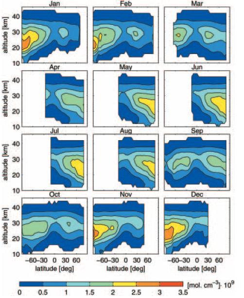
NOx from OSIRIS was merged with NOx from SAGE II to create a monthly mean time series, spanning from 1984 to 2018. For each instrument the NOx was derived from the retrieved NO2 and shifted to a local solar time of 12:00 pm using the PRATMO photochemical box model. The datasets were then debiased and merged by taking advantage of the 4-year overlap between the measurement periods.
Merged NOx from OSIRIS and SAGE II is available by following the directions under Download and navigating to the directory /Merged_Datasets/nox/
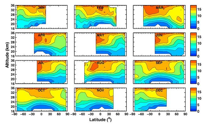
Stratospheric aerosol extinction climatology spanning from 2002 until May 2019. This product was constructed from the OSIRIS version 7 aerosol product. Extinction has been cloud-cleared as best as possible, but may underestimate extinction in fresh volcanic or wildfire plumes.
Climatology Grid:
- Latitude: 5 degree
- Longitude: 30 degree
- Time: Daily sampling with 5 day rolling average applied
- Altitude: 1 km
The climatology is available by following the directions under Download and navigating to the directory /OSIRIS/Level3/aerosol/7.0/
OSIRIS Level 1 Services
The OSIRIS Level 1 Spectrograph data product is only available for distribution by special request. If you would like more information on the OSIRIS Level 1 data, please contact Taran Warnock.
A sample of the OSIRIS Spectrograph data is available here.
The OSIRIS Level 1 InfraRed Imager System data product is only available for distribution by special request. If you would like more information on the OSIRIS Level 1 data, please contact Taran Warnock.
A sample of the OSIRIS IR data is available here.
Setup
These samples depend on xarray, numpy, scipy, and matplotlib. You will need the following imported into python to run the sample code below:
>>> import xarray as xr>>> import numpy as np>>> from scipy.interpolate import interp1d>>> import matplotlib.pyplot as plt>>> from matplotlib.colors import LogNorm
Spectrograph Data
If you have not already done so, download the sample OSIRIS Level 1 spectrograph data.
For example, you can access the data in orbit 54300 (the sample file) via:
>>> spect = xr.open_dataset('/path/to/OSIRIS_L1_Spectrograph_054300_2011-02-06_v2-0.nc')
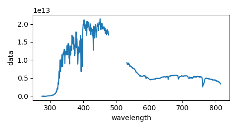
To plot a spectra (replacing pixel number with wavelength):
>>> spect.sel(time='2011-02-06T04:50:41.602559', method='nearest').swap_dims({'pixel': 'wavelength'}).radiance.plot(x='wavelength')
To plot a scan of spectrograph data:
>>> spect = xr.open_dataset('~/Downloads/OSIRIS_L1_Spectrograph_054300_2011-02-06_v2-0.nc')
>>> spect.where(spec.scan_number_time_dim == 54300021, drop=True).swap_dims({'time': 'tangent_altitude'}).sortby('tangent_altitude').radiance.plot(y='tangent_altitude', norm=LogNorm(1e9, 1e14))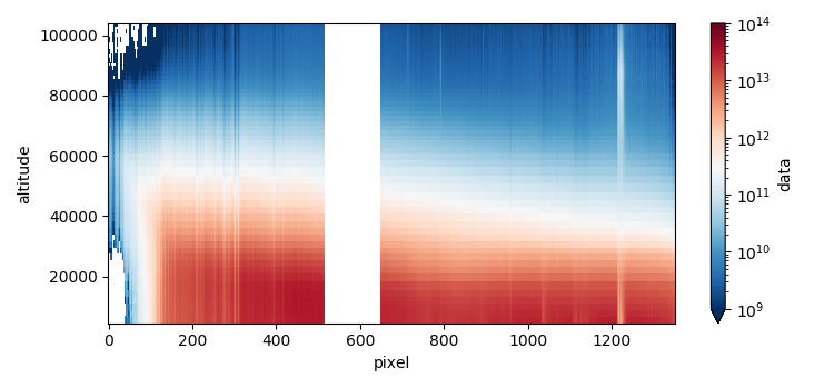
IR Data
If you have not already done so, download the sample OSIRIS Level 1 IR data. This data a sample orbit of channel 3 data for the IR instrument. It contains a single orbit of data with a daytime section in the middle and night time on either end. From left to right, the solar conditions are night, dusk, day, dawn, night. The zigzag motion of the data is due to the scanning nature of the spacecraft. That is, the satellite's attitude nods back and forth so that the instrument line-of-sight goes up and down the limb of the atmosphere. This allows the spectrograph (with its single line-of-sight) to scan the atmosphere from top to bottom. The IR instrument, on the other hand, has over 100 pixels that collect radiance data over ~100km span in the limb.
Access the IR data in orbit 36573 (the sample file) via:
>>> ir = xr.open_dataset('/path/to/ir_slc_036573_ch3.nc')
To plot the radiance data for the unmasked pixels. (noting the zigzag pattern in the data):
>>> ir.data.plot(x='time', y='pixel', norm=LogNorm(), vmin=3e8, vmax=1e14, figsize=(15, 6))
>>> plt.ylim(127, 15)
![]()
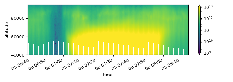
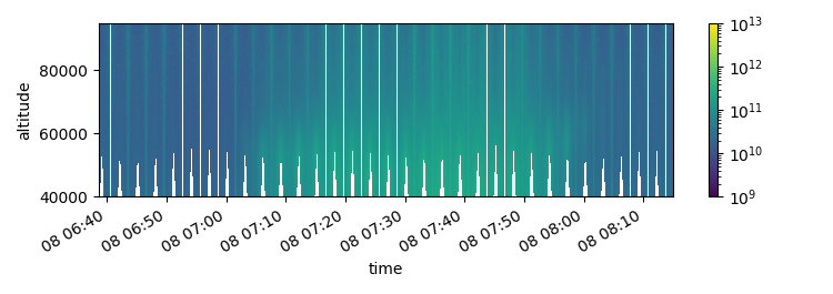
By interpolating to the attitude data contained within the file, we can view this data with respect to altitude and not pixel number:
>>> alts = np.arange(40000., 95000., 250.)
>>> ir_altitude = []
>>> for (data, alt) in zip(ir.data.transpose('time', ...), ir.altitude.transpose('time', ...)):
>>>     f = interp1d(alt, data, bounds_error=False)
>>>     ir_altitude.append(f(alts))
>>> ir_altitude = xr.DataArray(ir_altitude, coords=[ir.time, alts], dims=['time', 'altitude'])
>>> ir_altitude.plot(x='time', y='altitude', norm=LogNorm(), vmin=1e9, vmax=1e13, figsize=(15, 6))
Similarly the error estimate can be loaded and plotted via:
>>> alts = np.arange(40000., 95000., 250.)
>>> error_altitude = []
>>> for (error, alt) in zip(ir.error.transpose('time', ...), ir.altitude.transpose('time', ...)):
>>>     f = interp1d(alt, error, bounds_error=False)
>>>     error_altitude.append(f(alts))
>>> error_altitude = xr.DataArray(error_altitude, coords=[ir.time, alts], dims=['time', 'altitude'])
>>> error_altitude.plot(x='time', y='altitude', norm=LogNorm(), vmin=1e9, vmax=1e13, figsize=(15, 6))
SAGE III
The standard SAGE III/ISS NO2 retrieval neglects variations in solar zenith along the instrument's line of sight by assuming that the number density has a constant gradient within a given layer of the atmosphere. This assumption results in a retrieval bias for a species like NO2 that changes rapidly across the terminator.
A new algorithm was developed to account for these variations in the SAGE III/ISS NO2 by including a correction factor calculated with the PRATMO photochemical box model. The resulting SAGE III/ISS NO2 number density profiles can be downloaded by following the directions under Download and navigating to the directory (\SAGEIII_ISS\no2\Dube_2020\monthly).